1. What is Kalman Filter? The “Silent Hero” of Modern Navigation
2. Why use Kalman filter? Solving sensor noise and uncertainty IoT
3. Core Principles: How the Kalman Filter Algorithm Works Step-by-Step
4. Pros and Cons: Key Advantages and Limitations of Kalman Filters
5. Sensor Fusion in Action: Kalman Filter Applications in IoT and Autonomous Vehicles
6. Real-world Case Study
7. Conclusion: The Future of Precision Positioning in the IoT Era
1. What is a Kalman Filter? The “Silent Hero” of Modern Navigation
Have you ever wondered how your phone can still accurately pinpoint your location on a map even when the GPS signal is intermittent while navigating through tall buildings or tunnels? Or how a self-driving car can smoothly navigate its lane despite constant sensor vibrations? The answer behind these intelligent technologies is the Kalman Filter.
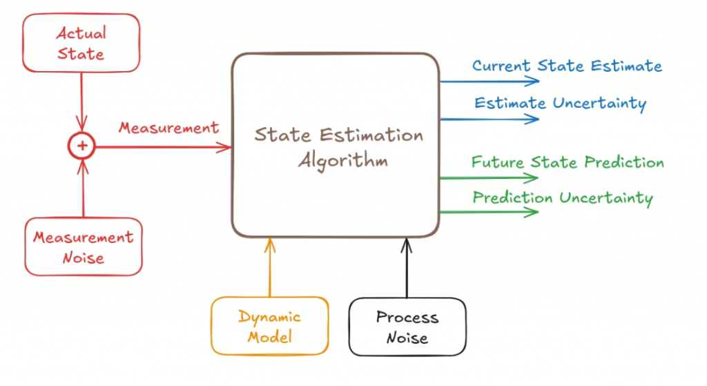
So what is a Kalman Filter? Simply put, it’s not a physical filter (like a water or air filter), but rather an intelligent mathematical algorithm that uses a series of measured values, affected by noise or error, to estimate a variable, thereby increasing accuracy compared to using only a single measured value. Its purpose is to help us “guess” (estimate) the true state of a system, even when the information we receive from sensors is noisy or not entirely accurate. It filters out “noise” from chaotic data to find the “true” signal.
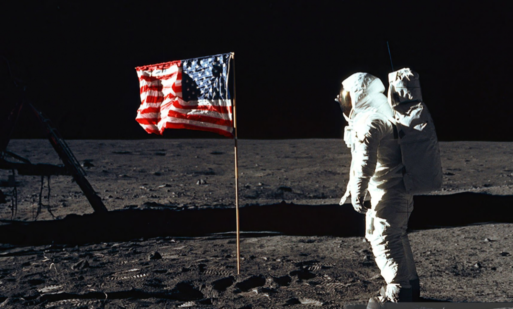
Twelve breathtaking minutes as humans landed on the Moon.
Do you know what this historic moment on the Moon, the smartphone in your pocket, and a modern self-driving car have in common?
They are all secretly using the same tool to answer the seemingly simple yet incredibly complex question: “Where am I in this chaotic world?”. It’s one of the greatest mathematical achievements of the 20th century, a “silent hero” behind most modern navigation technologies, yet its name is little known. Let’s uncover the secrets of the algorithm that took humans to the Moon and is guiding our future.
2. Why is a Kalman filter needed? To solve the problem of noise and uncertainty.
In an ideal technological world, if you want to know the position of an object, you simply use a measuring tape. But in the real world, nothing is perfect. The Kalman filter was created to address the core problem: uncertainty.
The practical problem: Sensor error and environmental noise
In an ideal technological world, determining the position of an object is simply a matter of using a measuring tape. However, the real world is never perfect, and we are always faced with the core problem of uncertainty. Any measuring device has an error margin; for example, the GPS on a phone can be off by tens of meters depending on the weather, or a temperature sensor can still fluctuate slightly even in a stable environment. No measurement is absolutely precise. Furthermore, constantly changing environmental factors such as wind, road friction, or engine lag make predicting movement difficult. If you rely solely on a single, often distorted, source of information, the result will be a erratic and inaccurate journey.
- Sensors are always subject to interference: Your phone’s GPS can be off by a few meters to tens of meters depending on weather conditions. Temperature sensors can fluctuate slightly even if the room temperature remains constant. No measurement is 100% accurate.
- The environment is constantly changing: Wind, road friction, engine lag… are external factors that make predicting the movement of an object difficult.
If you rely solely on a single source of information (for example, only on a GPS that’s experiencing interference), the result will be a choppy and inaccurate route.
The need for Sensor Fusion to optimize accuracy
To address this problem and optimize accuracy, engineers use the “Sensor Fusion” process to combine multiple different sources of information, and the Kalman filter is the most powerful tool for this. Imagine driving in thick fog: you have a predictive model based on maps and speedometers to calculate your position, but this calculation can be wrong due to slippery roads or wind. At the same time, you also have “measuring sensors”—faint road markers—but the fog makes you unsure if you’re seeing them correctly. At this point, the Kalman Filter acts as an intermediary “brain,” constantly evaluating whether to trust its own calculations more or those vague benchmarks. Based on the reliability of each source, it combines them to provide the best possible location estimate.
3. Core Principles: How the Kalman Filter Algorithm Works Step-by-Step
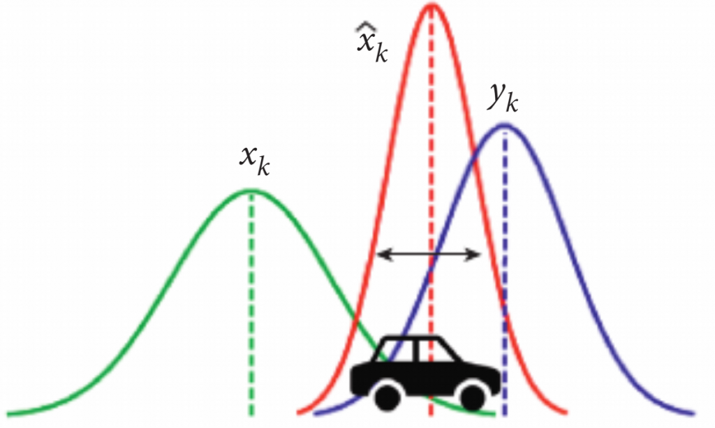
The Kalman filter never fully trusts anything. It operates based on a combination of mathematical modeling (prediction) and sensing (measurement).
Step 1: Prediction
The algorithm uses the physical state equation to shift the system from time t-1 to t.
- Logic: Based on the old velocity and position, it calculates the theoretical new position.
- Uncertainty: Due to external factors (system noise – Process Noise), the confidence probability range widens. This means that after each prediction step, we become less certain about the object’s exact position.
Step 2: Measurement
This is where raw data is collected from the sensors (GPS, Radar, Lidar).
- Logic: The sensor provides a direct observational value of the current state.
- Sensor error: Every measurement involves noise (Measurement Noise). This data is also represented by a probability distribution with its own standard deviation depending on the accuracy of the device.
Step 3: Correction/Update
This is the core logic of the algorithm, where the Kalman Gain (K) acts as the arbiter.
- Calculating K: This coefficient is determined by the ratio between the uncertainty of the forecasting model and the uncertainty of the sensor. If the sensor has low noise, K approaches 1 (the algorithm favors the measurement result). If the sensor has high noise, K approaches 0 (the algorithm favors the forecast result from the model).
- Optimal Estimate: This combination produces a new probability distribution with sharper peaks (smaller standard deviation) than both original data sources. This means the final result is more accurate than any single data source.

4. Pros and Cons: Key Advantages and Limitations of Kalman Filters
The Kalman algorithm has become an indispensable tool in modern engineering due to two outstanding advantages: mathematical optimization and computational efficiency. Theoretically, it has been shown to provide the best possible state estimation (with the smallest mean square error), provided the input assumptions are met. Besides accuracy, Kalman’s practical strength lies in its recursive nature. The algorithm doesn’t need to store entire cumbersome historical data sets; it only needs the immediately preceding state to compute the current step. This “lightweight” characteristic makes it extremely ideal for embedded computing systems with limited memory and power resources, such as in autonomous robots or handheld mobile devices.
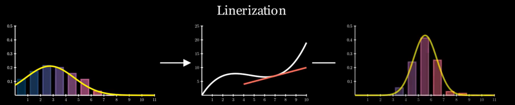
However, the standard (basic) Kalman filter is not a panacea due to significant limitations when applied to chaotic real-world scenarios. The biggest limitation is that it only works well with LINEAR systems, that is, systems that can be described by simple linear equations. Meanwhile, most real-world movements—for example, a robot performing a turn—are complex non-linear. Furthermore, this algorithm relies on the rigid assumption that system noise must follow a normal Gaussian distribution (bell-shaped). If the actual environmental noise has a different, unusual shape, the filter’s estimation efficiency will be severely degraded.
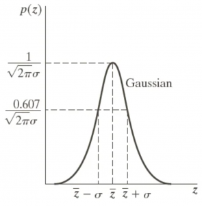
Gaussian Noise
To overcome the linearity barrier and bring the algorithm closer to practical applications, scientists have developed powerful upgraded versions. The most well-known and widely used solution is the Extended Kalman Filter, abbreviated as EKF. EKF handles nonlinear systems by applying local “linearization” techniques at each computation step, straightening complex curves to apply the basic Kalman mechanism. Thanks to this adaptability, EKF has now become an industry standard and is widely used in most advanced GPS and navigation systems today.
The Kalman Filter is considered one of the greatest algorithms of the 20th century, playing a core role in the Apollo moon landings and present in most modern rovers. To understand why this algorithm is so important yet so challenging, we need to consider two aspects: its superior computational capabilities and its stringent physical limitations.
Below is a detailed summary of the advantages, limitations, and potential extensions of the Kalman Filter:
Kalman Filter: Overview of Strengths and Limitations
5. Sensor Fusion in Action: Kalman Filter Applications in IoT and Autonomous Vehicles
The Kalman filter is one of the most widely used algorithms in engineering history.
- Applications in GPS Positioning and Navigation: On phones/cars, positioning systems often combine GPS (providing accurate location but slow updates and prone to signal loss) with inertial sensors (inertial meters, gyroscopes – very fast responses but prone to drift errors over time). The Kalman filter combines the advantages of both, providing smooth positioning even when the vehicle enters short tunnels.
- Key Role in Robotics and Autonomous Vehicles: Localization: Helps robots know their exact location on a surface map (SLAM); Object Tracking: Autonomous vehicles use Kalman to predict the movement of pedestrians or other vehicles on the road, thereby calculating a path to avoid collisions.
- Applications in Aerospace, Signal Processing, and Finance: Aerospace: Extremely important for determining the position and attitude of aircraft, rockets, and spacecraft. The Apollo program used Kalman filters in its navigation computers. Signal processing & finance: Used to smooth volatile stock market data or remove noise in audio and video signals.
Returning to the spacecraft mentioned above, this is where Kalman filters made their name.
When the Eagle module was only a few dozen meters from the lunar surface, the navigation computer (AGC) became overloaded and repeatedly reported the “1202 Alarm” error. In this context, the Kalman algorithm acted as the “silent brain” to process conflicting data streams to predict (a physical model). The computer calculated the trajectory of the fall based on the Moon’s gravitational pull and the thrust of the jet engines; then, using sensors and the landing radar, it continuously fired signals down to the surface to measure the actual distance and velocity. Finally, the radar data was heavily disrupted by the uneven terrain and blown-away lunar dust. If the radar had relied entirely on the data, the spacecraft would have made erratic engine adjustments and run out of fuel.
This is how Kalman handled it in those 12 seconds:
- Real-time noise filtering: The Kalman algorithm constantly compares: “The radar says it’s 5 meters away, but the physical model says it should be 7 meters.”
- Calculating Kalman Gain (K): Because the radar was experiencing interference at that time, the coefficient K automatically decreased. The algorithm “suspected” the radar and placed more trust in the stable orbital model.
- Optimal blending: Instead of jerky jumps between numbers, Kalman provided a smooth estimate, allowing Neil Armstrong to maintain stable control and steer the spacecraft away from large rocks, landing safely with only 25 seconds of fuel remaining.
6. Real-World Case Study
The story of Apollo 11 is not just a historical milestone; it also laid the foundation for modern navigation technology. Today, Kalman filters are no longer found in NASA’s massive computers, but are present in every smartphone, drone, and autonomous vehicle through the GNSS/INS integration model.
To understand why we need this combination, let’s look at the illustration of a GNSS satellite system (like GPS, GLONASS…). GNSS provides us with absolute positioning but has the disadvantage of slow update speeds and is prone to signal loss (when entering tunnels or tree canopies). In this case, the Kalman filter acts as the “conductor,” combining satellite data with an inertial navigation system (INS) – consisting of accelerometer and gyroscope sensors – to create a continuous and centimeter-accurate stream of positioning data.
To understand the power of the Kalman Filter, let’s consider a real-world car navigation system where it has to solve the problem of combining data from two sensor sources with contrasting characteristics:
- Accelerometer (INS): Extremely fast response to any change in motion, but if used for long-distance calculations, errors accumulate very quickly (drift).
- GPS (GNSS): Provides accurate absolute position and velocity over the long term, but the update rate is very slow (usually only once per second) and often experiences delays.
We will solve this problem in two stages (two consecutive Kalman loops):
Case 1: Velocity Estimation (A combination of “Quickness” and “Accuracy”)
In the integrated navigation system, the goal of Case 1 is to optimize instantaneous velocity estimation by combining two data sources with different noise characteristics, aiming for both responsiveness and system accuracy.
- Prediction Phase – Leveraging Dynamics: Using data from inertial sensors as input. Through the integration of the kinematic diagram, the filter provides a prediction of the velocity at time $k$. The advantage of this method is its high sampling frequency and instantaneous response to dynamic changes (acceleration, braking). However, due to the influence of white noise and bias, the integration process will cause cumulative error (drift), leading to a gradual deviation of the prediction value over time.
- Update Phase – Absolute Reference Correction: At this stage, the velocity from the GNSS receiver is used as a reference measurement (Observation). Although GNSS data is highly reliable in terms of absolute values, it is limited by the low update frequency and large signal delays due to satellite processing.
The Kalman Filter’s optimization mechanism:
The algorithm balances the two data sources using the Kalman Gain. When the vehicle undergoes a sudden change in state, the difference between the accelerometer prediction and the actual GNSS measurement increases. The Kalman filter analyzes the covariance of the error to determine the weighting:
- In dynamic state: When there is a large change in acceleration that the GNSS hasn’t updated in time due to delay, the filter will temporarily increase the weighting of the accelerometer prediction model, helping the system track the actual velocity trajectory without data lag.
- In steady state: The filter will prioritize data from GNSS to “anchor” the velocity value, while estimating and eliminating the accelerometer polarization error, preventing data drift.
Result: The output of Case 1 is an optimal velocity estimate with smooth, high bandwidth characteristics and no cumulative error. This is the pure input variable for the position estimation model in the next stage.
Case 2: Estimating Location/Distance (Utilizing the results of Case 1)
After obtaining the optimal velocity vector from Case 1, the goal of this phase is to determine the precise spatial coordinates of the vehicle using a second-stage Kalman filter (Cascaded Kalman Filter).
- Prediction Phase – Smooth Trajectory Interpolation: The system uses the “clean” velocity estimate from the output of Case 1 as the input variable to perform position integration. Based on a dynamic state-space model, the filter predicts the vehicle’s next position at a high frequency (e.g., 100Hz). Thanks to the use of the denoised and biased velocity from the previous step, the predicted trajectory becomes extremely smooth, eliminating the “jump” in position often seen in devices using only GNSS.
- Update Phase – Coordinate Anchoring Correction: Absolute coordinates (Longitude, Latitude) from the GNSS system are used as a correction measurement. This is a source of “ground truth” data to control errors. Although the velocity integration in the prediction step was very good, mathematically, even the smallest errors will accumulate over time (Integration Drift). The coordinate points from the GNSS act as absolute “anchors” to reset these errors.
The role of the Kalman Filter in trajectory optimization: The algorithm performs Sensor Fusion at a more complex level:
- Maintaining Continuity: In scenarios of temporary satellite signal loss (e.g., a vehicle entering a tunnel or under dense foliage), the Kalman filter relies entirely on the predicted model from the velocity in Case 1 to “continue” the trajectory. This capability helps the system maintain continuous navigation without interruption.
- Smoothing Data: When a new GNSS signal (which often has noise of a few meters) is detected, the filter does not immediately jump to the new location. Instead, it calculates the difference between the predicted and measured location (Innovation), then subtly adjusts the estimated location through the weights of the covariance matrix.
Overall result: Through a two-stage Kalman filter structure, the system achieves optimal convergence: providing position and velocity with high temporal resolution (from INS) and consistently high absolute accuracy (from GNSS). This is the core principle that enables autonomous vehicles and guided missiles to operate stably in the most dynamically complex environments.
7. Conclusion: The Future of Precision Positioning in the IoT Era
The Kalman filter is proof of the power of mathematics in conquering chaotic realities. From the historic Apollo missions to today’s era of autonomous vehicles, this algorithm remains the “soul” that helps positioning systems achieve absolute accuracy through its ingenious Sensor Fusion mechanism.
In short, mastering the Kalman filter is key to creating groundbreaking IoT products—where smoothness and accuracy are paramount. This is not just technology, but the foundation for a safer and smarter automated future.